Dense Vector Search: How Semantic Search Works
Dense vector search is the backbone of modern semantic retrieval. Every document gets encoded as a 768-number vector. At query time, the query is encoded the same way, and the system finds the nearest document vectors. "Cheap phones" finds "affordable smartphones" because they occupy the same region of vector space.
The pipeline
Documents → Preprocess → Embed → Index (HNSW)
Query     → Preprocess → Embed → kNN search → Ranked results
Four steps. Same embedding model at both index time and query time — this is non-negotiable.
Step 1: Preprocess
Clean text consistently before embedding. Inconsistent preprocessing causes silent recall degradation:
- Strip leading/trailing whitespace
- Collapse multiple spaces into one
- Remove markup and formatting artifacts
- Truncate or chunk to model's max token limit (typically 512 tokens)
For long documents, chunk with overlap. A 2,000-word article becomes four 500-word chunks with 50-word overlaps. Store each chunk with a reference back to the source document.
Step 2: Embed
Generate a normalized vector for each chunk. Normalization to unit length (L2 norm = 1) ensures cosine similarity equals dot product, which vector indexes compute faster.
Batch documents together during indexing — processing 32 documents at once is significantly faster than 32 individual calls.
Step 3: Index
Once vectors are generated, load them into a vector index with HNSW:
Create collection with:
  - dimension = 768 (must match embedding model output)
  - distance  = cosine
  - M         = 16
  - ef_construct = 256

Upload points (id, vector, payload):
  - payload stores title, text, domain, tags
  - payload enables filtered search without embedding metadata
Index build time scales roughly linearly with corpus size. A 1M-document corpus takes 30–45 minutes to index.
Step 4: Search
At query time:
1. Preprocess query text (same pipeline as documents)
2. Embed query with the same model
3. Send query vector to index with limit=10
4. Optionally apply payload filters (domain, difficulty, date)
5. Return scored results
Pre-filtering (applying filters before kNN traversal) is more efficient than post-filtering when the filter is selective. If a filter removes more than 30% of the corpus, pre-filter.
Performance benchmarks
On a 1M document corpus at 768 dimensions:
| Metric | Value |
|---|---|
| NDCG@10 | 0.85 |
| P95 search latency | ~45ms |
| Memory footprint | ~3 GB |
| Index build time | ~40 min |
| Throughput | ~22 QPS (single thread) |
What dense search gets right
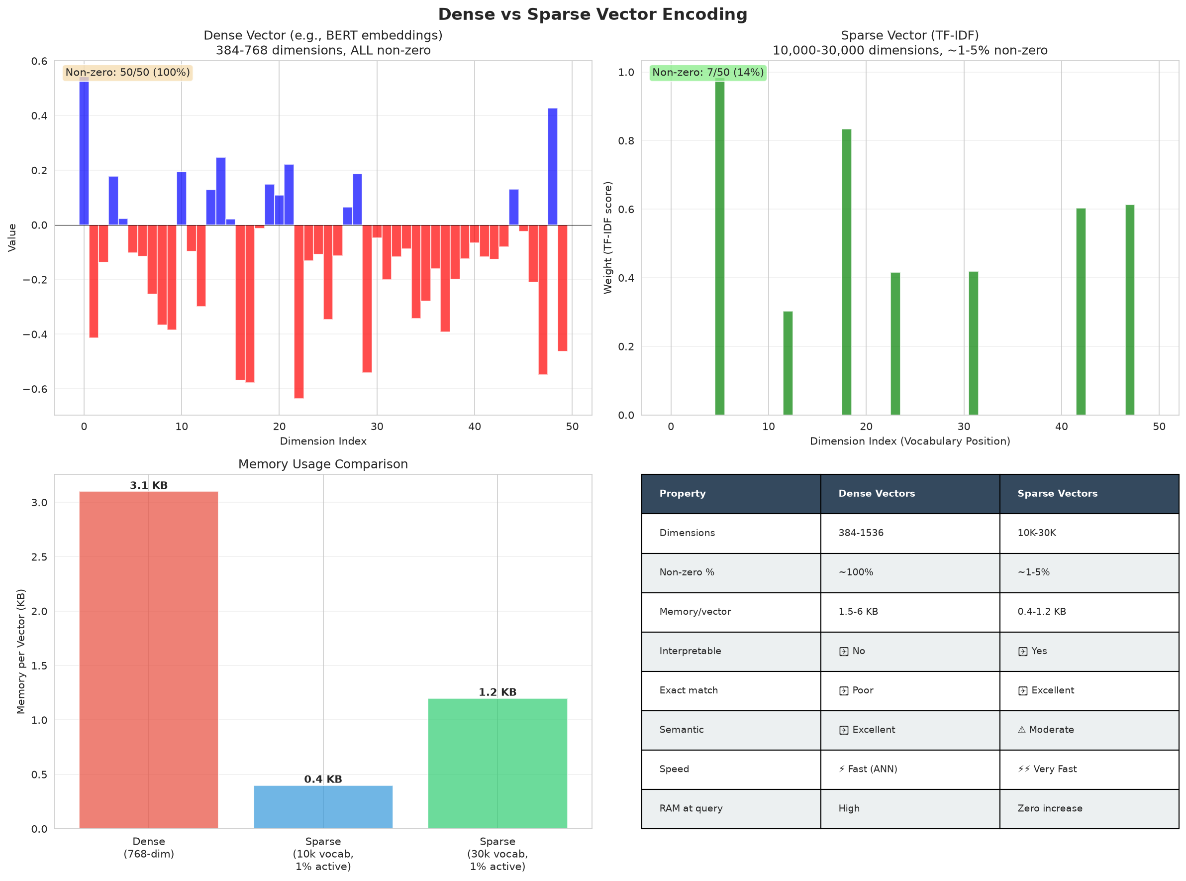
Dense search excels when meaning varies from phrasing:
| Query | Dense result | Why it works |
|---|---|---|
| "affordable smartphone" | Finds "cheap phone" articles | Synonym handling |
| "heart disease treatment" | Finds "cardiac care" articles | Concept mapping |
| "how to speed things up" | Finds "performance optimization" | Intent understanding |
| Multi-language query | Finds results in any language | Cross-lingual embeddings |
NDCG@10 by query type:
- ▸Synonym queries: 0.91
- ▸Concept queries: 0.93
- ▸Exact term queries: 0.68 ← weakness
Where dense search fails
Run these against a pure dense search system and watch it struggle:
- ▸Exact IDs: "order-123456" returns semantically similar orders, not the exact one
- ▸Error codes: "NullPointerException line 47" matches "null reference" articles instead of the specific error
- ▸Technical jargon: "RFC 2822 date format" may miss the exact specification article
- ▸Precise measurements: "64GB RAM" matches "large memory" content instead of the specific spec
NDCG@10 for exact-term queries: 0.68 vs 0.85 overall. For applications where these queries matter, dense search alone is not enough.
[Key Insight] The failure mode of dense search is invisible — it returns something plausible, not nothing. Users see results that look reasonable but aren't what they actually needed. This is harder to debug than a keyword search returning zero results. Always benchmark your specific query distribution, not just aggregate NDCG.
The pre-filtering vs. post-filtering decision
Pre-filter (filter → kNN): efficient when the filter is selective. The index only traverses the filtered subset. Use when > 30% of documents are excluded.
Post-filter (kNN → filter): simple but wasteful. Fetch more results than needed (limit × 3–5), then filter. Use only for loose filters.
Never embed metadata into vectors as a workaround for filtering — it makes re-indexing expensive and pollutes the embedding with non-semantic signals.
Relevance tuning checklist
When results aren't good enough, work through these in order — most problems trace back to one of them:
- ▸
Chunk size and overlap — this is the #1 lever. Too-small chunks lose context; too-large chunks dilute the relevant signal. Start at 400–500 words with 50-word overlap. If recall is low on long-form content, increase chunk size and overlap until chunks capture complete ideas.
- ▸
ef_search — if your index recall (measured against exact kNN ground truth) is below 95%, increase ef_search. This is a runtime change — no re-indexing needed.
- ▸
k oversampling for reranking — retrieve top-50 or top-100 candidates from the vector index, then apply a reranker to return the true top-10. The vector index finds candidates; a reranker finds the best among them.
- ▸
Switch to hybrid — if pure dense search is missing exact-term queries, adding keyword search is almost always the right fix. A single dense index can't learn to handle both semantic and exact-match queries well simultaneously.
- ▸
Embedding model quality — if none of the above help, the model may not represent your domain well. Evaluate domain-specific models, or fine-tune on your corpus with a contrastive objective.