kNN and HNSW: How Vector Search Scales
Finding the nearest vector in a corpus of 1 million documents sounds simple. The naive implementation — compare your query to every document — is called exact kNN. It's 100% accurate. It's also unusable at scale.
At 768 dimensions and 1M vectors, exact kNN computes 768M multiply-add operations per query. On commodity hardware that's ~45ms per query, giving you about 22 queries per second. A production search system needs 200–500 QPS minimum.
HNSW (Hierarchical Navigable Small World) solves this by building a graph that lets you skip most comparisons. It achieves 95–99% recall at 10–100× the throughput.
Exact kNN: the baseline
Exact kNN scores every document against the query and returns the top k. It's O(n) — query time grows linearly with corpus size.
| Corpus size | Exact kNN latency |
|---|---|
| 1,000 docs | ~1ms |
| 100,000 docs | ~100ms |
| 10,000,000 docs | ~10,000ms |
This is why you need approximate search at any meaningful scale.
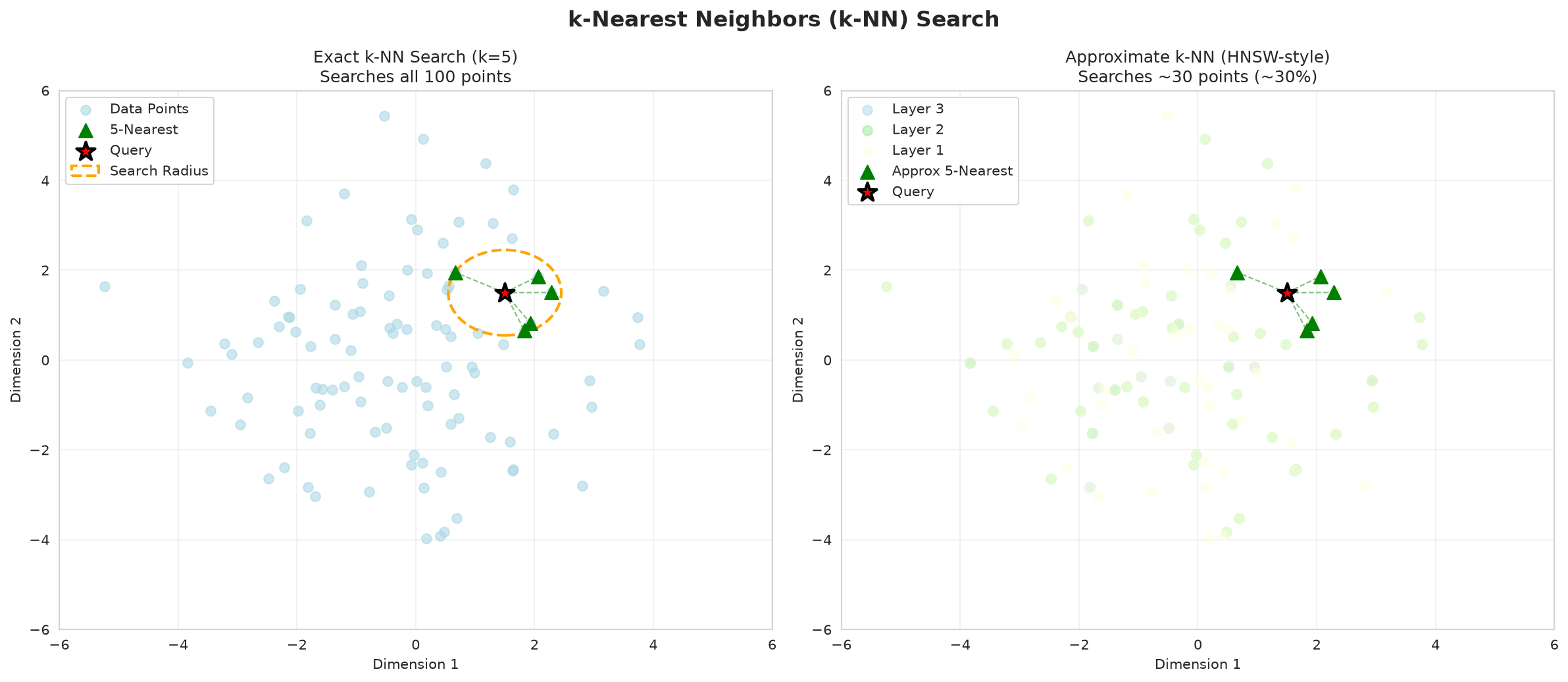
HNSW: the idea
HNSW builds a graph where each node (document vector) is connected to its nearest neighbors. A query traverses this graph greedily — always moving to a neighbor closer to the query — until it can't improve.
The "hierarchical" part adds multiple layers with different densities:
- ▸Top layers: sparse, long-range links — fast global navigation
- ▸Bottom layer: dense, local links — precise final neighborhood
A query enters at the top, locates the rough neighborhood quickly, then descends to refine.
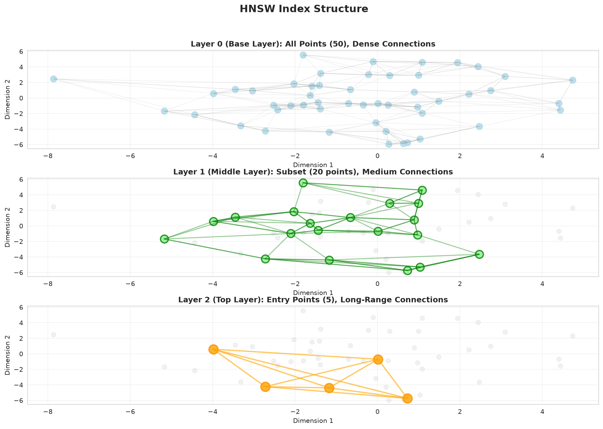
Layer 2 (5 entry points):  A ─────────────── E
Layer 1 (20 points):        B ─── C ─── D ─── E
Layer 0 (all points):       A─B─C─D─E─F─G─H─I─J
                                  ↑
                         query descends here for final precision
How the HNSW graph is built
Understanding index construction helps you reason about why tuning parameters matter:
- ▸Initialization — start with an empty graph (or the existing one for incremental updates)
- ▸Entry point — the top layer serves as the global starting point for all insertions
- ▸Adding a new vector — for each new document, the algorithm:
- ▸Starts at the top layer and greedily navigates toward the new vector
- ▸At each layer, selects up to
Mnearest neighbors to connect to - ▸Uses
ef_constructas the size of the candidate list considered at each layer — higher ef_construct means more candidates examined, producing better-quality edges - ▸Some connections span layers, creating "shortcuts" that dramatically speed up traversal
- ▸Graph pruning — after bulk insertions, the graph can be optimized to improve navigability and remove redundant edges
The key insight: the graph is built greedily, not globally optimally. Two vectors that should be neighbors might not be connected if they were inserted far apart in time. Higher ef_construct reduces this problem by considering more candidates during each insertion.
How HNSW search works step-by-step
At query time, the traversal mirrors the build process in reverse:
- ▸Enter at the top layer — start from the global entry point
- ▸Greedy descent — at each layer, move to whichever neighbor is closest to the query vector
- ▸Priority queue — maintain a candidate list of size
ef_search; update it as better neighbors are found - ▸Refine at lower layers — each descent finds a progressively closer neighborhood
- ▸Return k results — stop when the desired number of nearest neighbors are identified
The ef_search parameter is the size of this priority queue. Larger queue = more candidates explored = higher recall, but more work per query.
The three parameters that matter
M — max connections per node
Each node stores M bidirectional links. Higher M = better recall + more memory per node. The default value of 16 is right for most use cases. Use 32 for applications where recall above 98% is critical.
ef_construct — build-time search width
During index construction, each node evaluates ef_construct candidates before selecting its M best links. Higher ef_construct = better index quality + longer build time. 256 is a good production default.
ef_search — query-time search width
At query time, the graph explores ef_search candidates before returning k results. This is your runtime lever — increase it when recall is too low without having to rebuild the index.
The recall vs. latency tradeoff
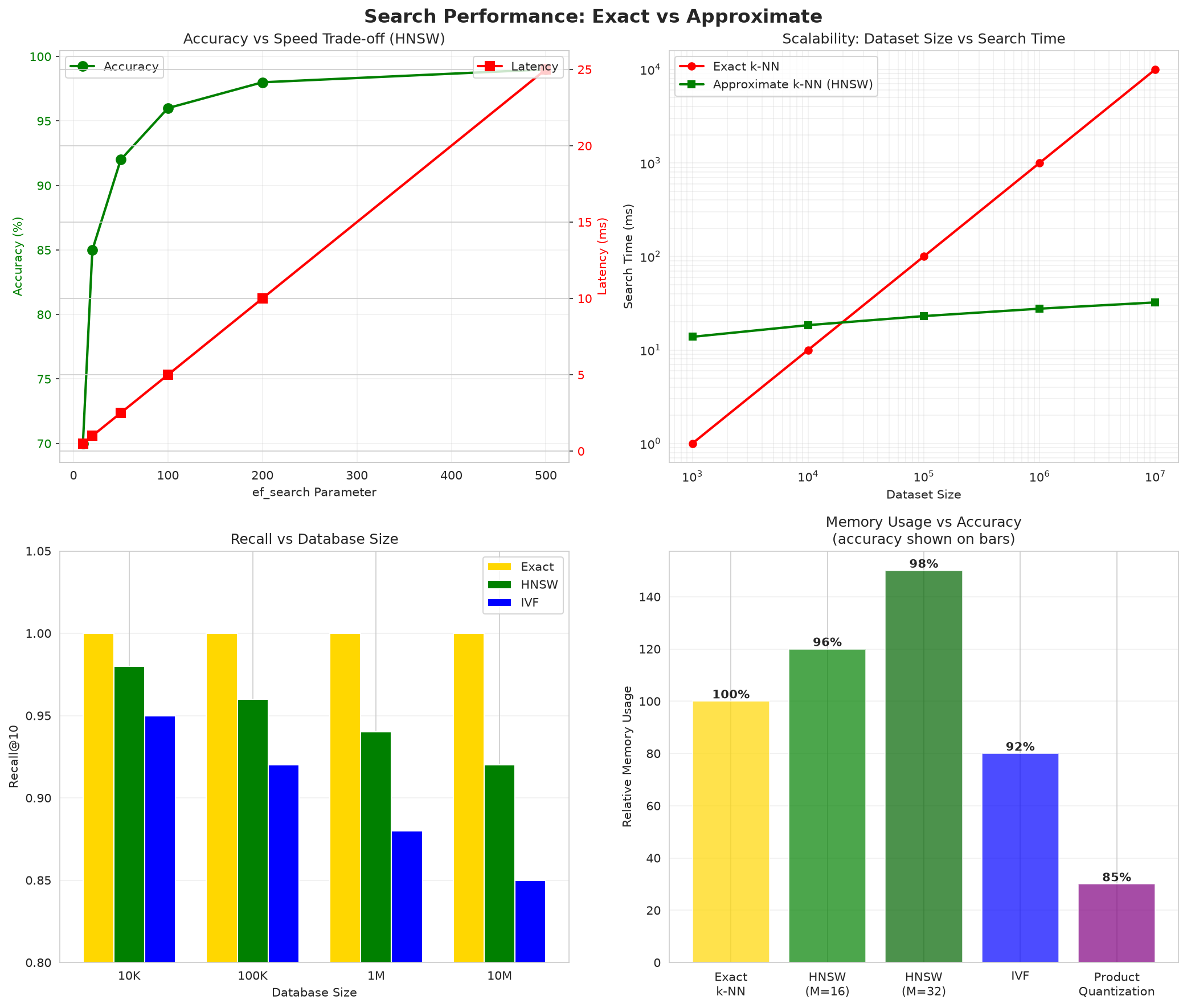
| ef_search | P95 latency | Recall@10 | Use case |
|---|---|---|---|
| 50 | ~25ms | 92% | High-volume, latency-sensitive |
| 100 | ~50ms | 96% | Production default |
| 200 | ~100ms | 98% | High-precision applications |
| 500 | ~250ms | 99% | Research / offline evaluation |
[Key Insight] Start with ef_search = 100 in production. Measure recall against a ground truth sample (run exact kNN on a representative query set, compare top-10 results). Only increase ef_search if recall is measurably impacting user outcomes — the latency cost of 96% → 99% recall is often not worth it.
Scalability
HNSW's O(log n) complexity means latency barely grows as the corpus scales:
| Scale | Exact kNN | HNSW | Speedup |
|---|---|---|---|
| 1K vectors | 1ms | 2ms | 1× |
| 100K vectors | 100ms | 5ms | 20× |
| 10M vectors | 10,000ms | 15ms | 667× |
Memory footprint
Each node stores its vector plus M × 2 link pointers:
memory per doc = (dims × 4 bytes) + (M × 2 × 4 bytes)
               = (768 × 4) + (16 × 2 × 4)
               = 3,072 + 128  = ~3.2 KB

1M docs = ~3.2 GB
Apply INT8 quantization to reduce vector storage 4×: ~1 GB for 1M docs instead of 3.2 GB.
Exhaustive kNN: not just for small corpora
Exact kNN has one use case beyond small datasets — building ground truth for recall evaluation.
To measure how well your HNSW index is performing, you need to know what the correct answers are. Exhaustive kNN gives you the globally exact top-k for every query in your test set. You then compare HNSW results to those exact results and compute recall:
Recall@10 = |results_HNSW ∩ results_exact| / 10
This is how the benchmarks in this article were produced. Run exhaustive kNN on a sample of 500–1,000 queries, collect ground truth, then measure HNSW recall across different ef_search values to find your operating point.
HNSW fields can also be queried exhaustively on demand (without a separate index) using a query-time flag — useful for debugging specific bad results without rebuilding anything.
When HNSW is the wrong choice
HNSW works well for static or append-heavy corpora where you can build the index once and serve it. It struggles with:
- ▸Frequent deletes: requires soft-delete + periodic re-index to avoid "tombstone" degradation
- ▸Very small corpora (< 10K docs): brute-force exact kNN is simpler and fast enough
- ▸Streaming ingestion at high velocity: live graph updates are expensive; batch and rebuild instead
For write-heavy workloads, inverted file (IVF) index variants — which partition the space into clusters and search only relevant clusters — can be a better fit.