Sparse Encoding: Fast, Interpretable, and Underrated
Dense vectors compress meaning into 768 floats — every dimension is active, and none of them map to anything human-readable. Sparse vectors take the opposite approach: they have 50,000+ dimensions, but 99.97% are zero. The non-zero dimensions correspond to actual terms in your vocabulary.
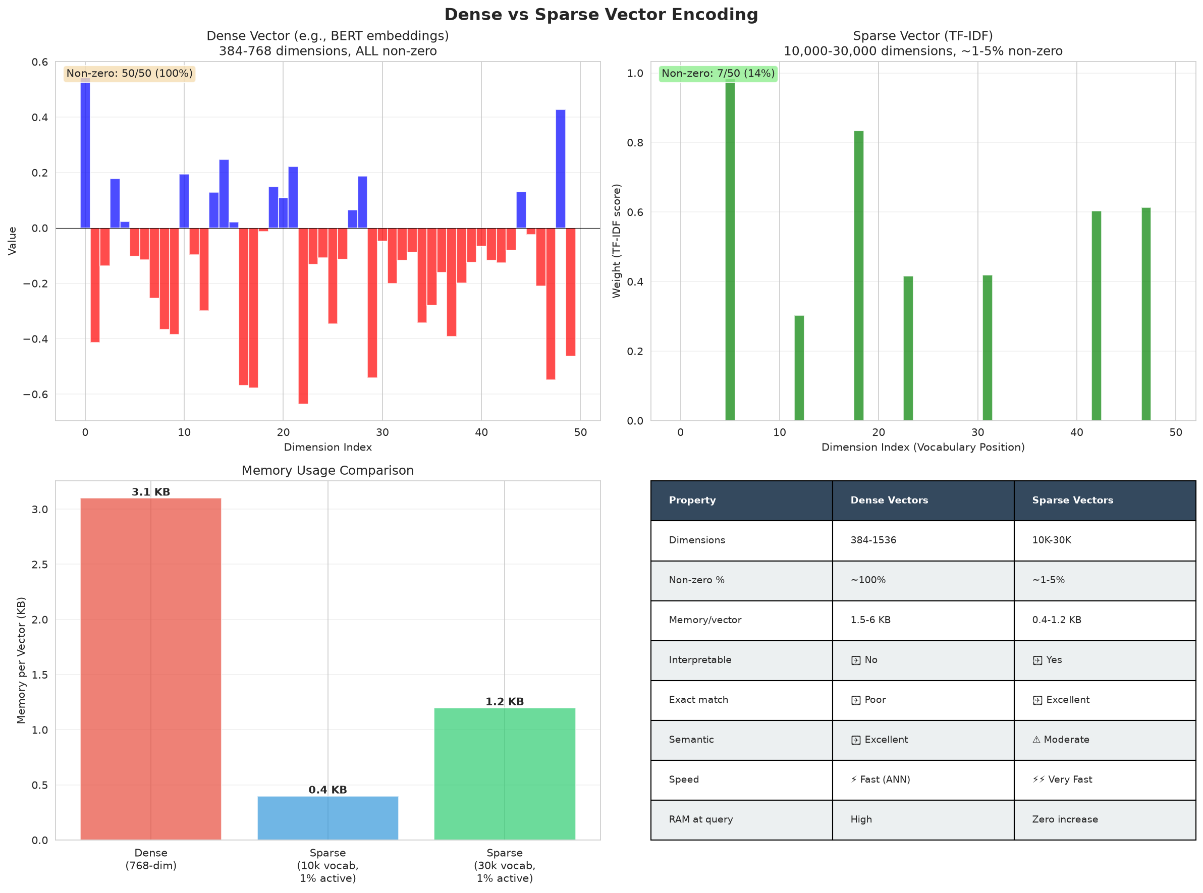
Dense vector for "expensive smartphone":
  [0.23, -0.87, 0.41, 0.12, ...]   ← 768 opaque floats, all non-zero

Sparse vector for "expensive smartphone":
  {
    "expensive":  0.85,
    "smartphone": 0.79,
    "phone":      0.52,
    "device":     0.31,
  }   ← 4 of 50,000 possible terms active, rest are zero
You can read a sparse vector and understand exactly what it says. That interpretability is a production advantage — debugging bad results is far easier when you can see which terms drove a match.
How sparse encoding works
TF-IDF (Term Frequency–Inverse Document Frequency) is the foundation:
TF(term, doc)  = how often this term appears in this document
IDF(term)      = log(total_docs / docs_containing_term)
TF-IDF(t, d)   = TF × IDF
High IDF = the term is rare across the corpus → it's distinctive. High TF = the term appears frequently in this document → it's important here. A term that appears in every document (like "the") has IDF ≈ 0 and contributes nothing.
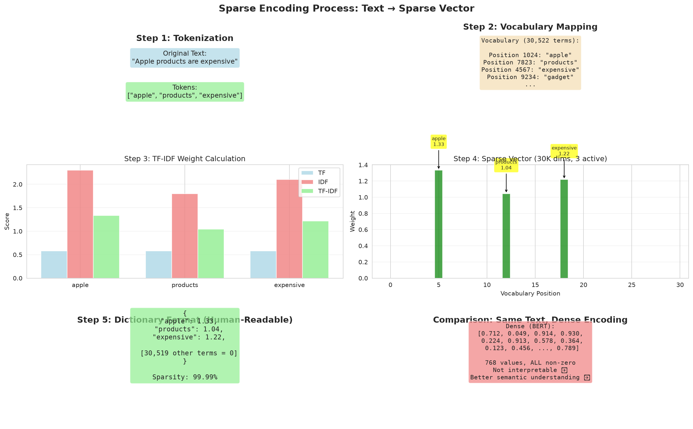
The full pipeline:
- ▸Tokenize the text
- ▸Remove stop words
- ▸Calculate TF per document
- ▸Calculate IDF across corpus
- ▸Multiply TF × IDF
- ▸L2-normalize the resulting vector
- ▸Store only non-zero values (the sparse representation)
Why sparse search is 10x faster
Dense similarity requires a dot product across all 768 dimensions — one number per dimension per document.
Sparse similarity only processes overlapping terms:
Query:    {"expensive": 0.85, "smartphone": 0.79}
Doc A:    {"expensive": 0.72, "phone": 0.54}       ← 1 overlap
Doc B:    {"laptop": 0.88, "screen": 0.61}          ← 0 overlaps, skip entirely
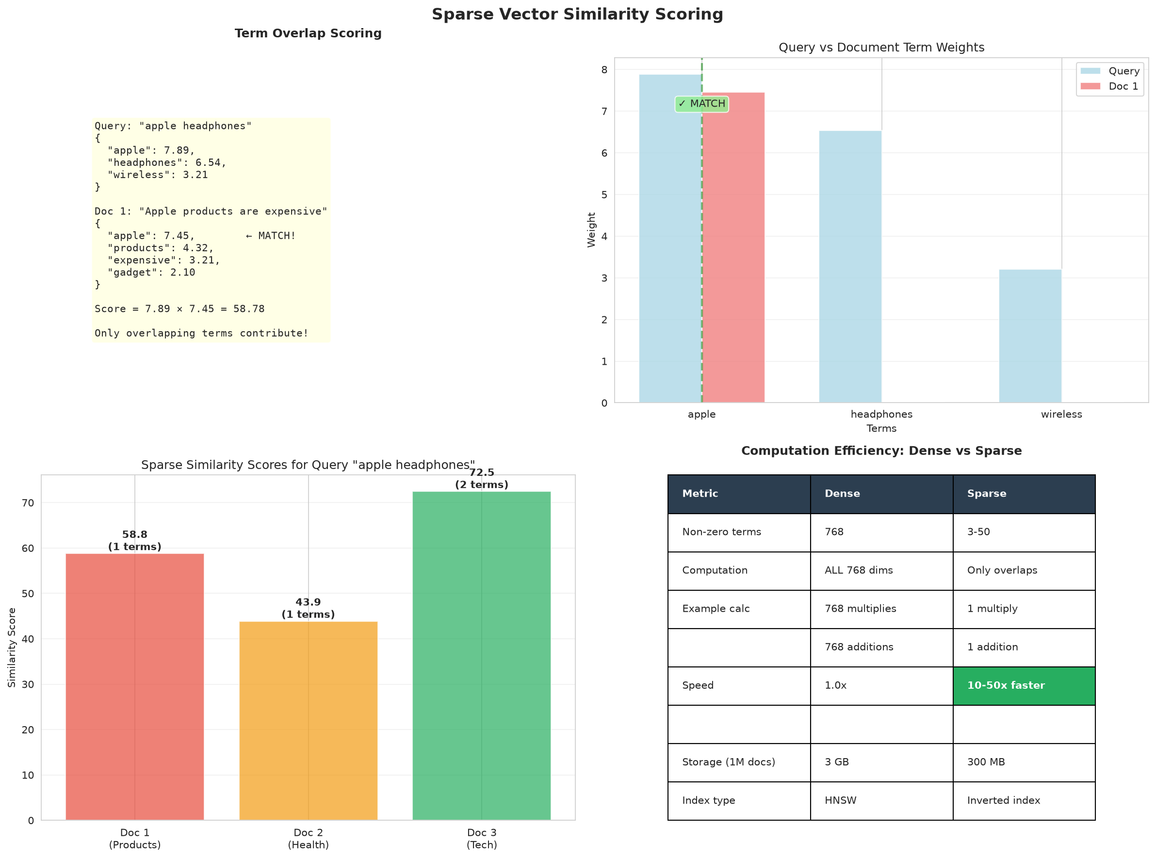
Documents with zero query-term overlap are never touched. In practice, a query with 5 terms overlaps with only ~0.1% of a large corpus — the other 99.9% are skipped entirely. This is why sparse search is 10× faster:
| Method | P95 latency | Memory (1M docs) |
|---|---|---|
| Dense (768d) | 45ms | ~3 GB |
| Sparse (TF-IDF) | 5ms | ~300 MB |
When sparse beats dense
| Query type | Dense NDCG@10 | Sparse NDCG@10 | Winner |
|---|---|---|---|
| "affordable smartphone" (synonym) | 0.91 | 0.52 | Dense |
| Exact product code "SKU-12345" | 0.68 | 0.89 | Sparse |
| Technical term "NullPointerException" | 0.64 | 0.84 | Sparse |
| Conceptual "heart disease" | 0.93 | 0.47 | Dense |
| Log trace ID search | 0.30 | 0.95 | Sparse |
Sparse wins on controlled vocabularies: product SKUs, error codes, function names, legal case numbers, log trace IDs — any query where the user knows the exact term.
[Key Insight] Use sparse search when your users search with terms from a controlled vocabulary: catalog codes, error strings, API method names, specification numbers. These are tokens that dense vectors encode poorly because they're treated as rare or unknown during embedding model training.
Learned sparse expansion
Standard TF-IDF fails on synonyms: the word "expensive" doesn't expand to "costly". Learned sparse models fix this by adding weighted related terms at reduced weight:
Base encoding:       {"expensive": 0.85, "smartphone": 0.79}

After expansion:     {"expensive":  0.85,
                      "smartphone": 0.79,
                      "costly":     0.43,   ← added at 50% weight
                      "pricey":     0.43,   ← added at 50% weight
                      "phone":      0.37}   ← added at lower weight
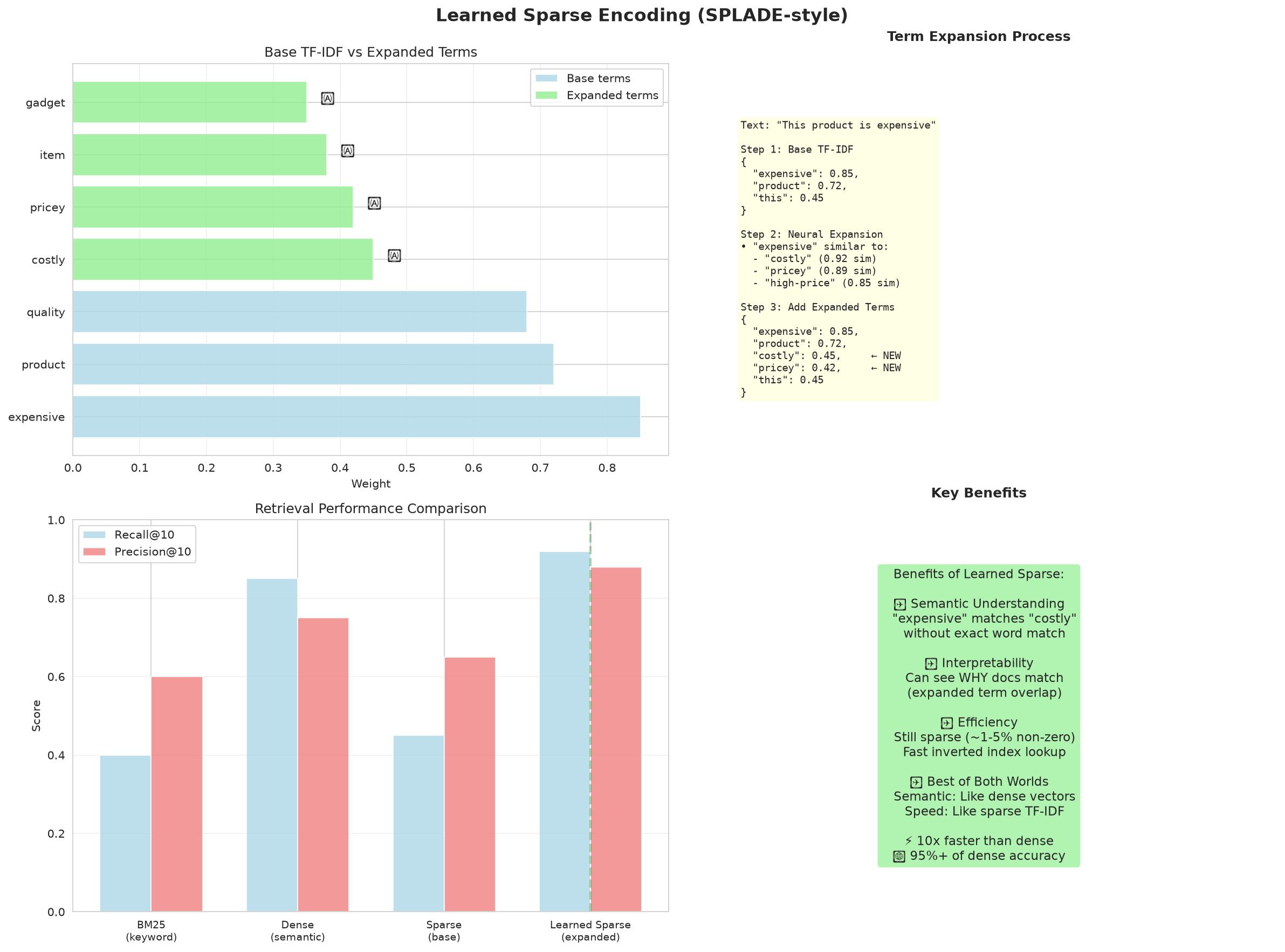
Expansion factor (typically 0.3–0.5) controls how aggressively synonyms are added. Too high and you lose the precision advantage of sparse; too low and recall doesn't improve.
Models trained end-to-end for sparse expansion (like the SPLADE family) consistently outperform manual synonym dictionaries because they learn domain-specific relationships from data.
Best use cases for sparse encoding
- ▸E-commerce: SKU search, exact product name match
- ▸Technical documentation: function names, configuration keys, error codes
- ▸Legal and compliance: case numbers, statute citations, exact terminology
- ▸Log search: trace IDs, IP addresses, structured log fields
- ▸Medical records: ICD codes, drug names, procedure codes
All of these share one property: users know exactly what they're looking for, and the terms are precise.